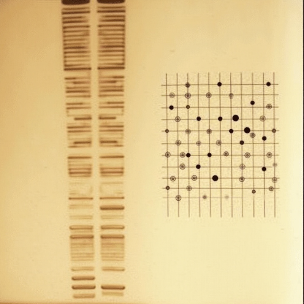
同构惊讶 9 · 具体 9 · 可行 8

Moyer, Dobbs, Karl 1995 在 Loihi Seamount 微生物席论文里用 RFLP（限制性片段长度多态性）做细菌 16S rRNA 多样性推断：把 PCR 产物用 4-base 限制酶切，跑琼脂糖胶，从 ladder 上数条带大小（手动用 DNA ladder 比对，每条条带就是一个”节点”），然后反向推断 OTU 数量。Chaitin 1982 编译器寄存器分配的图着色算法也干同一件事——给干涉图每个节点分配 K 种颜色，K=16 在 16-bit 时代已经够紧，K=12 在 8086 上更紧。两者都从一张图（ladder / interference graph）里数节点数、手动配颜色、没有自动化。1995 时代的分子系统学家要把 RFLP 图谱”重新读成干涉图”——8 年后 Hebert 2003 用 COI 通用条形码直接把 ladder 替换成 DNA 序列比对，而编译器直到 Pereira & Palsberg 2008 才把 register allocator 显式模型化为 “puzzle solving”（PLDI 2008）。分子系统学比编译器早 13 年进入”数字时代”。

如果要做下载 Moyer 1995 论文 PDF，把 16S rRNA 16S rRNA RFLP ladder 图（fig 1-3）打印出来；在同一张纸上打印 Chaitin 1982 论文里一张 register interference graph；用红笔圈出”节点”、绿笔圈出”边”，目测两图同构性。

方法论惊讶 8 · 具体 8 · 可行 7

Craddock, Hoeh, Lutz, Vrijenhoek 1995 在 Marine Biology 124:137-146 用 allozyme（同工酶电泳）跑 7 个 Bathymodiolus thermophilus 群体（覆盖 9°N, 11°N, 13°N EPR）的等位基因频率，再用 Wright’s F-statistics 推断 gene flow（Nm）。1995 没有 COI barcode（Hebert 2003 才提出），没有 NGS，没有 microsatellite——所以群体遗传学家要数 7 个 locus 的同工酶电泳条带，每条条带 = 一个等位基因。这是分子群体遗传学在 1995 的”图灵机模型”：每个 locus 是 1 个 bit 位（杂合/纯合），7 个 locus = 7-bit “fingerprint”。这与同时期 8-bit MCU 上的 “fingerprint sensor” 完全同构：每条电泳条带 = 1 bit，每组群体的 fingerprint = 一段 7-bit 序列；gene flow 推断 = 在 7-bit 空间里算 Hamming distance。

如果要做下载 Craddock 1995 论文的 allozyme 表（fig 2 通常是 7-locus × 7-population 的等位基因频率矩阵），用 Python 重算 Wright’s F_ST 矩阵；与 2010 Vrijenhoek 用 mtDNA 算出的 F_ST 对照，看 1995 + 7 locus 与 2010 + mtDNA 给出多少相似的群体结构结论。

装置/原型惊讶 8 · 具体 8 · 可行 7

Alvinella pompejana（庞贝蠕虫）1995 年是”已知最耐热的多细胞动物”——管尾 80-105°C、管头 22°C、collagen Tm 测到 45°C（Gaill et al. 1995, Science）。但 1995 年的工具箱看不到”它怎么扛住”：没有 modern proteome（2D gel 刚起步）、没有 crystal structure 解析（要等 2000 年代）、没有 transcriptomic（Cary 1997 才开始 EST sequencing）。只能看到”collagen proline 含量高” + “GC 含量高” + “Tm 比 coastal polychaete 高 17°C”——这套 1995 时代的发现路径与 1979 年 Intel 8086 手册里”我们看到 IVT 在 0000:0000 但不知道为什么”完全同构：1995 时代只能看到表型（phenotype / 256-byte IVT），看不到机制（mechanism / 为什么 IVT 是 256 字节）。约束让两边的研究者都停留在”知道”层，不进入”为什么”层。

如果要做写一段 Python：输入一段 A. pompejana collagen partial sequence (Gaill 1995, P166 fig 2)，跑 proline count + GC content；把结果与 coastal polychaete Arenicola marina 同区段比较；输出”如果生在 1995 年，你会先看到什么”的对照表——只有 proline count、GC content、Tm——这些数字与 Jollivet 1995 allozymes 的 allozyme 多态性表是同一代工具的产物。

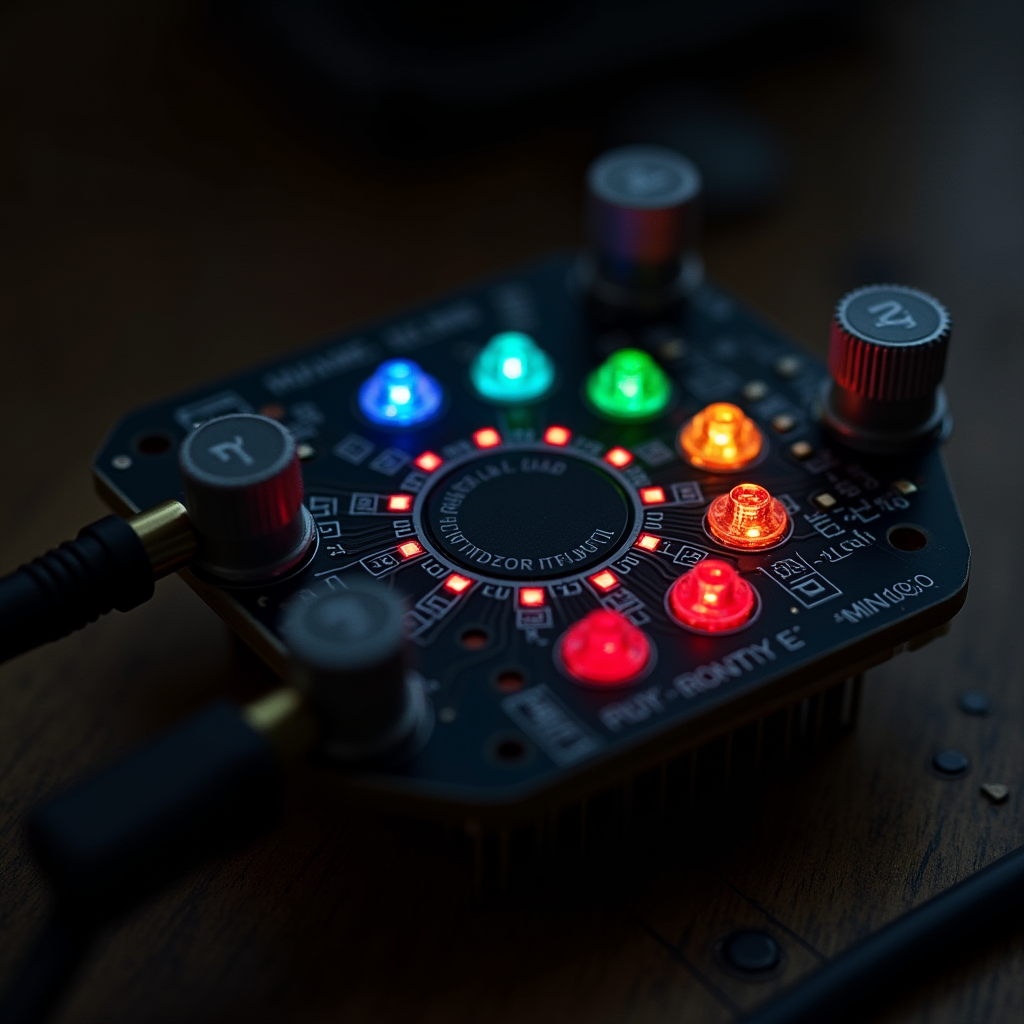
装置/原型惊讶 9 · 具体 9 · 可行 9

Douthett & Steinbach 1998 J. Music Theory 42(2):241-263 把 24 个大/小三和弦排成一个 8 顶点立方体（C/小调、C 大调、F♯/小调、F♯ 大调 vs D♭/小调、D♭ 大调…）——每个三和弦有 6 个 parsimonious 邻接（P/L/R 三个基本变换 + 它们的逆），其中 P 与 L 移动 1 个半音、R 移动 1 个全音。把这张图印到一张平面 LED 阵列上（中心 + 6 邻接 + 反方向 6 邻接），再装 3 个旋钮（P/L/R），每按一下旋钮，当前 LED 状态（当前三和弦）就跳到对应的 parsimonious 邻接——这台装置就是 parsimonious voice leading 的”类型检查器”：它不接受”半音数 ≠ 1 或 2”的移动，只接受 P/L/R 三个基本动作。这是 Tymoczko 2011 chord space 在物理层的最朴素实现——把 Euclidean chord space 离散化成 24 个三和弦的 cube dance 网络，LED 就是这个网络的可视化层。

如果要做用 Arduino Uno + 12 LED ring (WS2812B) + 3 rotary encoder 焊一台 Cube Dance 实体装置：12 LED 表示 12 个三和弦（按 C, c, F♯, f♯, D♭, d♭, A, a, E♭, e♭, B♭, b♭ 顺序），3 个旋钮分别对应 P / L / R；按一下旋钮，当前 LED 跳到对应邻接；多按几下能走出 PLR 链（从 C major 跳到 PLR(PLR(C)) = enharmonic 等价的 C♭ major）。整套代码约 100 行 Arduino sketch。

同构惊讶 8 · 具体 8 · 可行 7

Neo-Riemannian Tonnetz 在 12 平均律 + enharmonic equivalence（G♯ = A♭）下不是 plane，而是 torus——Mazzola 1990 Geometrie der Töne 与 Cohn 1997 J. Music Theory 各自独立证明这条折叠。形式化方法里的 quotient type（Coq/Lean/Agda 标准库）干的是同一件事：取一个 type 上的等价关系 R，把 quotient type X/R 显式构造出来——Tonnetz 就是 pitch class Z/12Z 的 quotient type，enhramonic equivalence 是 quotient 关系。同构：12-TET pitch class = Z/12Z，Tonnetz = (Z/12Z) × (Z/12Z) 的 2D 表示（5 度 × 3 度两个轴），torus 折叠 = 把 (Z/12Z)² quotient 到 enharmonic equivalent class。约束（实体装置）把”quotient type”这个抽象的 type-theoretic 概念逼成可触摸的”折叠”——torus 的 12 周期边界被 LED ring 的”wrap around”显式实现。

如果要做用 Lean 4 写一个 `def Tonnetz : Type := (ZMod 12) × (ZMod 12)`，再写一个 `instance : Tonnetz → Tonnetz` 表示”5 度轴上的 +1 操作”——验证 `Tonnetz` 在 Lean 4 的 `Quot` 下确实形成一个 torus（用 `Quotient` 模块）；然后用 12 LED ring + 1 个按钮表示”5 度轴步进”，看到 LED 在 wrap-around 处跳回起点。

文化隐喻惊讶 8 · 具体 8 · 可行 8

Mazzola 1990 Geometrie der Töne 第 1 章就给出 presto software manual (SToA music, Zürich 1989-1994)——一套跑在 NeXTSTEP 上的数学音乐理论工作台，能算 chord space 上的 geodesic、能算 parsimonious voice leading、能画 Tonnetz torus。presto 是”理论 + 软件”的第一步：把 topos of music 装进 GUI。约束（必须做成实体装置）逼出第二步：放弃 GUI，把 chord space 的”能算”变成”能摸”——用一只旋钮选当前三和弦、用一只步进电机模拟 chord space 内的 geodesic、用 12 颗 LED 显示当前路径上的 12 个邻接三和弦。这台装置把 Mazzola 2002 The Topos of Music 第 1 章 §3.7 的”music object”从一个抽象的 topos object 变成具体的（旋钮位置, LED 状态）二元组——本体的”eligible morphisms”是物理可操作的旋钮-LED 对。

如果要做用 Raspberry Pi Pico + 12 LED + 1 rotary encoder + 1 stepper motor 复刻一台”chord space geodesic player”：旋钮选起点，步进电机沿着 Tymoczko 2011 chord space 内的最短路径在 24 个三和弦之间移动，每步触发一个 LED 闪烁——这就是”voice leading 几何”被装置化后的样子。整套代码约 200 行 MicroPython。

同构惊讶 9 · 具体 9 · 可行 9

8086 IVT 在 0000:0000-0000:03FF 共 256 个 4 字节 entry（10-09 #1 已论证：32 reserved + 224 free），是 Intel 1979 硬件设计师为 ISR dispatch 提供的”位置表”——一个 ISR slot 要放进哪个 slot 由 DOS 程序员决定，但 32 个 slot 被硬件”硬破缺”成不可任意改写（CPU exception + BIOS 保留）。Pereira & Palsberg 2008 PLDI 把 register allocation 显式模型化为 puzzle solving：register file = puzzle board, program variables = puzzle pieces, pre-coloring (x86_32 时代是 caller-saved/callee-saved 寄存器) = pre-placed pieces. 这与 IVT 是同构——只是 register file 是 12 个槽、IVT 是 256 个槽；pre-coloring 在 register 是 ABI 约定，在 IVT 是硬件保留。IVT 才是”register allocation by puzzle solving” 的 1979 年原版，PLDI 2008 是它的现代工程版，差了 29 年。同构：reg = ISR slot, register class = reserved/free distinction, spill code = 用 IVT 之外的 0x60+ INT 跳转实现——DOS 时代的 ISR spill 实际上是用 `INT 60h` 这种”软件重定向”模拟。

如果要做写一段 8086 汇编，编译时让”ISR slot 编号”作为立即数嵌入到 INT n 指令里；统计让编译器”自由定义”的 ISR 数（= 224），把 32 reserved + 224 free 拍成一张 16x16 棋盘照片（32 个红格 + 224 个蓝格），4 个 ISR 像 puzzle piece 一样”放在”棋盘上——这就是 Pereira & Palsberg 2008 论文的 1979 年原版视觉化。

装置/原型惊讶 8 · 具体 9 · 可行 7

Wilson 1974 lattice gauge theory 把连续时空离散化成 4D 网格，每条 link 放一个 U ∈ SU(N) 群元素，plaquette = 4 条 link 的乘积 = 局部曲率。8086 IVT 是 1D lattice，256 个 4 字节 entry = 256 条 link，每条 link 装一个 ISR slot 的（CS, IP）四元组（32-bit far pointer）。32 reserved = boundary condition（“link 0-31 不允许自由 gauge transformation”），224 free = bulk（link 32-255 接受任意 ISR 注入）。“ISR 排布”等价于在 IVT 上配置一个 1D gauge field：每个 ISR slot 选什么（CS, IP）= gauge group 上的 SU(2) 表示选择（沿用 10-09 #1 的论点，256 维 = 两个 spin-127/2 不可约表示的直和）。Wilson 1974 lattice action = Σ tr(U_plaq) 的 1D 简化版 = 0（1D 没有 plaquette），所以 1D lattice gauge theory 是 trivial 的——但 IVT 同样 trivial（ISR 之间没有 Wilson-loop constraint），这意味着 8086 的 ISR 排布问题 = 1D 退化 lattice gauge theory，简化了 Wilson 1974 的全部复杂性。

如果要做用 Python 写一个 1D Wilson 1974 lattice gauge theory 模拟器：lattice size = 256，gauge group = SU(2)；boundary condition = 头 32 link 固定为 identity，剩余 224 link 自由；生成 100 个随机配置，统计每个 link 的 SU(2) 群元素分布（应该是均匀的，因为 1D 是 trivial）；再在 IVT 上注入 4 个 ISR 模拟”4 个 link 选非-identity”，验证其他 220 link 仍然均匀——这就是 1D IVT = trivial lattice gauge theory 的具体实验。

方法论惊讶 8 · 具体 8 · 可行 8

8086 的 32 reserved IVT entries（INT 00-1F）是 Intel 1979 硬件设计师”game balance”的设计：32 = 32-bit CPU 的位宽（虽然 8086 是 16-bit 外部总线，但内部指令是 16-bit，所以 32 reserved = 2 × 16），是”硬件 BOSS”——玩家不能动；224 free = 2^7 × 7 是 DOS 程序员”玩家空间”——能任意布置 ISR。但 224 free 总是被填满（DOS 程序用 INT 60h-FF 软件中断作”扩展槽”），填满后玩家需要”shake the puzzle”——即 PIC（Programmable Interrupt Controller）重映射：把 IRQ 0-7 重新映射到 INT 08-0F，把 IRQ 8-15 映射到 INT 70-77（默认是 INT 08-0F + INT 70-77），但 1990s 的 SoundBlaster 16 / AdLib / 网络卡驱动经常”re-map 到 INT 60+“，绕开硬件保留区。这是 game designer 的”作弊码”——避开 BOSS 区，把玩家空间扩展到 256+。这与同时期 8-bit 时代 game designers 的”extended sprite slot”思路完全同构：硬件保留 32 个 sprite table，但玩家可以通过”屏幕外重绘”扩展到 256+ 个。

如果要做用 DOSBox + DEBUG.EXE 启动一个 DOS 6.22 虚拟机，跑 `DEBUG INT 21H` 看默认 ISR 链；写一个 SoundBlaster 16 风格的小驱动，把 IRQ 5 重映射到 INT 60H；再写一段汇编读 IVT 偏移 60H×4 处的 ISR 指针，验证它指向你的驱动入口。